Even most adult brains follow the same principle when they observe something new. At the time of observation, they retain this new information in their memory as postulations – “may be this is a peach” (language text) or “may be the boy is playful” (causal reasoning) or “may be this is Mr. Smith” (knowledge), until their postulations are confirmed by a trusted source, often in the nearest-neighbor. These observations and confirmations happen in two different time-points. And, sometimes the observed postulations are radically altered with the confirmation of new information – “oh no, this is an apricot, not peach” (language text) or “no, the boy is sarcastic, not playful” (causal reasoning) or “ah, this is Mr. David, not Mr. Smith” (personality) – at the time of confirmation. In this learning process, the former is proactive learning whereas, the latter – retroactive learning – changes the original postulations or replaces the deep-seated beliefs through new information connections, often either guided by experience or information from the nearest-neighbor or both.

So, what happens to state of the information between proactive and retroactive – two different time points – in the learning cycle? The neuroscience research has shown that in early childhood, and again in the teens and subsequently at various stages of learning, brains go through bursts of refinement, forming and then optimizing the connections in the brain. Connections determine what the subject or object is, what does it do, and how does it do. Early childhood provides an incredible window of opportunity with neural connections forming and being refined at such an incredible rate, there isn’t a certain time when babies are learning – they are always learning. Every moment, each experience translates into physical trace, a part of the brain’s growing network. One of the most powerful set of findings concerned with the learning process involves the brain’s remarkable properties of “plasticity” – to adapt, to grow in relation to experienced needs and practice, and to prune itself when parts become unnecessary – which continues throughout the lifespan, including far further into old age than had previously been imagined. The demands made on the human learning are key to the plasticity – the more one learns, the more one can learn – and, therefore required to be included in this architecture of artificial neural network for machine learning.

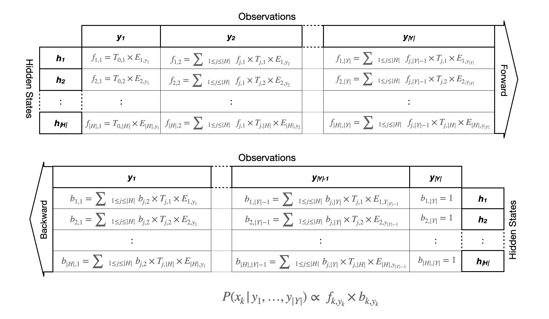
The forward-backward algorithm is a splitting method for solving  inference in both hidden Markov models (HMMs) and conditional random fields (CRFs). Conditional Random Field (CRF) is the statistical and computational framework that allow for modeling linear chains and more complex sequentially dependent events. In forward algorithm (as the name suggested), we use the computed probability on current time step to derive the probability of the next time step. This is used to calculate a ‘belief state’ – the probability of a state – at a certain time, given the history of evidence. It computes the posterior distributions of all hidden state variables given a sequence of observations. Hence the it is computationally more efficient. Backward Algorithm is the time-reversed version of the forward algorithm. In backward algorithm we find the probability that the machine will be in hidden state at time step t and will generate the remaining part of the sequence of the visible symbol. We often need to do further inference on the sequence. For example, we may wish to know the likelihood that observation x_i in the sequence came from state k i.e. P(π_i = k | x). This is the posterior probability of state k at time step i when the emitted sequence is known.

When learning from long sequences of observations the FB algorithm may be prohibitively costly in terms of time and memory complexity. However, alternative technique is include approximating the backward variables of the F-B algorithm using a sliding time window on the training sequence, or slicing the sequence into several shorter ones that are assumed independent, and then applying the FB on each sub-sequence (we discussed this in other sections later). This employs the inverse of HMM transition matrix to compute the smoothed state densities without any approximations. A detailed complexity analysis indicates that this technique is more efficient than existing approaches when learning of HMM parameters form long sequences of data.

In stochastic differential equation (SDE), in simpler form called arithmetic Brownian motion used by Louis Bachelier as the first model for stock prices in 1900, known today as Bachelier model. In a partial differential equation (PDE) that describes the time evolution of the probability density function of the velocity of a particle under the influence of drag forces and random forces, as in Brownian motion. In a real-valued continuous-time stochastic process (the Wiener process), sometimes one actually has the final condition and want to work out its initial. It is common in financial derivatives, where one knows the payoff or reward function at maturity, have a model for the dynamics of its underline asset and want to know the initial price of the derivative. So one needs to work in reverse, this is the backward stochastic differential equation (BDSE) – as a pair of adapted processes such that, with the terminal condition, for given adapted stochastic process coefficient, n-dimensional Brownian motion, and measurable random variable.